Day 5: Perceptrons in Python from Scratch. (Code)
Perceptron implementation in Python from scratch using PyTorch and SkLearn.
Jun 05, 2021
Perceptrons are building blocks of Neural Networks. In this blog post, we will do an implementation of classic Rosenblatt Perceptron from scratch in PyTorch. If you need a refresher then go through this article to get an idea about the maths behind this.
I chose to use PyTorch instead of NumPy because it is widely used in the deep learning community. All the blog posts in the 100 Days of Deep Learning project will be mostly covered using PyTorch only.
Wanna jump right to code, check out complete code on Github.
Perceptron code implementation in Python using PyTorch.
The very first thing we need to create a Perceptron implementation is a dataset. We use the amazing Scikit Learn library to create a custom dataset.
Do bear in mind that Perceptron can only do binary classification that is why create a dataset for classification.
We create a dataset of 100 features of two different types (100 - 100 each). We split the dataset into a 70/30 ratio for training and testing.
X, y = datasets.make_blobs(n_samples=100, n_features=2, centers=2, cluster_std=1.05, random_state=6)
X = torch.from_numpy(X)
y = torch.from_numpy(y)

X_train, X_test = X[:70], X[70:]
y_train, y_test = y[:70], y[70:]

# Normalize (mean zero, unit variance)
mu, sigma = X_train.mean(axis=0), X_train.std(axis=0)
X_train = (X_train - mu) / sigma
X_test = (X_test - mu) / sigma

fig = plt.figure(figsize=(10, 8))

plt.plot(X_train[:, 0][y_train == 0], X_train[:, 1][y_train == 0], 'r^')
plt.plot(X_train[:, 0][y_train == 1], X_train[:, 1][y_train == 1], 'bs')
plt.xlabel("feature_1")
plt.ylabel("feature_2")
plt.title('Binary data')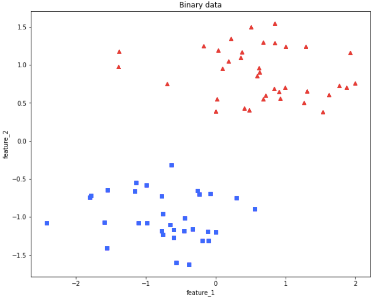
You can see from the above visualization of training data, we have two different classes.
print('Feature count', torch.bincount(y))
print('X shape:', X.shape)
print('y shape:', y.shape)

#Output
Feature count tensor([50, 50])
X shape: torch.Size([100, 2])
y shape: torch.Size([100])
Perceptron Model class
Next, we define a perceptron model. We define 4 main methods in this class namely
- forward
- backward
- train
- evaluate
def custom_where(cond, x_1, x_2):
    return (cond * x_1) + (~(cond) * x_2)

class Perceptron():
    def __init__(self, num_features: int):
        self.num_features = 2
        self.weights = torch.zeros(num_features, 1, dtype=torch.float32)
        self.bias = torch.zeros(1, dtype=torch.float32)

    def forward(self, x):
        linear = torch.add(torch.mm(x, self.weights), self.bias)
        predictions = custom_where(linear > 0., 1, 0).float()
        return predictions

    def backward(self, x, y):
        predictions = self.forward(x)
        errors = y - predictions
        return errors

    def train(self, x, y, epochs):
        for e in range(epochs):
            for i in range(y.size()[0]):
                errors = self.backward(x[i].view(1, self.num_features), y[i]).view(-1)
                self.weights += (errors * x[i]).view(self.num_features, 1)
                self.bias = errors

    def evaluate(self, x, y):
        predictions = self.forward(x).view(-1)
        accuracy = torch.sum(predictions == y).float() / y.size()[0]
        return accuracy
Once we have declared out model we run the code by creating a object of Perceptron class. Let's see what it gives out in terms of Weights and Bias.
ppn = Perceptron(num_features=2)

X_train_tensor = X_train.clone().detach().type(torch.FloatTensor).to('cpu')
y_train_tensor = y_train.clone().detach().type(torch.FloatTensor).to('cpu')

ppn.train(X_train_tensor, y_train_tensor, epochs=5)

print('Model parameters:')
print('  Weights: %s' % ppn.weights)
print('  Bias: %s' % ppn.bias)

# Output
Model parameters:
  Weights: tensor([[-0.2096],
        [-2.2456]])
  Bias: tensor([0.])
Next we check the accuracy of the model on test dataset.
X_test_tensor = X_test.clone().detach().type(torch.FloatTensor).to('cpu')
y_test_tensor = y_test.clone().detach().type(torch.FloatTensor).to('cpu')

test_acc = ppn.evaluate(X_test_tensor, y_test_tensor)
print('Test set accuracy: %.2f%%' % (test_acc*100))

# Output
Test set accuracy: 100.00%
Great job!
Our model has achieved 100% accuracy on our dataset. This means from the complete dataset even on the test_dataset which we have not used to train the Perceptron model has achieved 100% accuracy.
Visualization
Let us visualize this to view how our model is classifying the input.
##########################
### 2D Decision Boundary
##########################

w, b = ppn.weights, ppn.bias

x_min = -2
y_min = ( (-(w[0] * x_min) - b[0])
          / w[1] )

x_max = 2
y_max = ( (-(w[0] * x_max) - b[0])
          / w[1] )


fig, ax = plt.subplots(1, 2, sharex=True, figsize=(9, 4))

ax[0].plot([x_min, x_max], [y_min, y_max])
ax[0].title.set_text('Training dataset [70%]')
ax[1].plot([x_min, x_max], [y_min, y_max])
ax[1].title.set_text('Test dataset [30%]')

ax[0].scatter(X_train[y_train==0, 0], X_train[y_train==0, 1], label='class 0', marker='o')
ax[0].scatter(X_train[y_train==1, 0], X_train[y_train==1, 1], label='class 1', marker='s')

ax[1].scatter(X_test[y_test==0, 0], X_test[y_test==0, 1], label='class 0', marker='o')
ax[1].scatter(X_test[y_test==1, 0], X_test[y_test==1, 1], label='class 1', marker='s')

ax[1].legend(loc='upper left')
plt.show()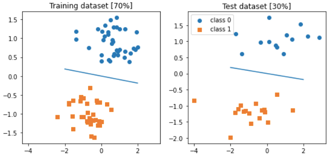
The visualizations are for training data and testing data respectively. You can view from the visualization above that model is making a clear distinction between both the classes. This shows that 100% accuracy achieved by the model is indeed right.
Conclusion
We created a very basic Perceptron model from scratch and achieved 100% accuracy on our dataset. I suggest running the code on your machine by yourself and tinker with the dataset and model to see how it performs in different cases.
Get the complete code on GitHub.