Day 7: Perceptrons from scratch using NumPy.

Perceptron implementation from scratch using NumPy and Matplotlib. Dataset via Scikit Learn.

By Nandeshwar

Jun 07, 2021

Perceptron algorithm is a building block of Neural Networks. In this notebook, we implement the Perceptrons in NumPy and plot using matplotlib.

Perceptron Algorithm in NumPy and Matplotlib

Check out this article for Perceptron implementation in PyTorch.

Perceptron algorithm is a building block of Neural Networks. In this notebook, we implement the Perceptrons in NumPy and plot using matplotlib.

Perceptron is denoted as

$$
\begin{aligned}
W_{x} + b = \sum_{i=1}^{n} w_{i} + b \\
\end{aligned}
$$

Step Function

Above output is passed through this step function

"Yes" if $ W_{x} + b \geq 0 $ else "No"

Assumptions

Binary classification dataset.
Labels are only 0 and 1.
Weights are denoted by W.
Labels are denoted by y.
Features are denoted by X.
Learning rate is denoted by $ \alpha $.

Pseudocode for Perceptron Algorithm Implementation.

Initialize random weights $ W_{1}, W_{2}, W_{3} .... W_{n} $.
For every mis-classified point $ X_{1}, X_{2}, X_{3} .... X_{n} $.
    If prediction=0:
        For i=1,2....n:
            Change $ W_{i} + \alpha*X_{i} where \alpha $ is learning rate
        Change $ b = b + \alpha $
    If prediction=1:
        For i=1,2....n:
            Change $ W_{i} - \alpha*X_{i} where \alpha $ is learning rate
        Change $ b = b - \alpha $

Wanna jump right to code, check out complete code on Github.

Import libraries

import numpy as np
import pandas as pd
from sklearn import datasets

import matplotlib.pyplot as plt

%matplotlib inline
plt.rcParams['figure.figsize'] = [10, 7]

Create and Visualize Data

X, y = datasets.make_blobs(n_samples=100, n_features=2, centers=2, cluster_std=1.05, random_state=6)

plt.plot(X[:, 0][y == 0], X[:, 1][y == 0], 'r^')
plt.plot(X[:, 0][y == 1], X[:, 1][y == 1], 'bs')
plt.xlabel("feature_1")
plt.ylabel("feature_2")
plt.title('Binary data')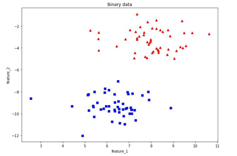

You can see from the above visualization of training data, we have two different classes.

StepFunction

Step function changes the value to 0 and 1 to which is their actual label.

Prediction

We calculate the value with Weights and Bias learned.

Perceptron

This is where we update the weights and biases based on their final value.

def stepFunction(t):
    if t >= 0:
        return 1
    return 0

def prediction(X, W, b):
    return stepFunction((np.matmul(X,W)+b)[0])

def perceptronStep(X, y, W, b, learn_rate = 0.01):
    for index in range(len(X)):
        y_hat = prediction(X[index], W, b)
        if y_hat-y[index] == 1:
            W[0] -= X[index][0] * learn_rate
            W[1] -= X[index][1] * learn_rate
            b -= learn_rate
        elif y_hat-y[index] == -1:
            W[0] += X[index][0] * learn_rate
            W[1] += X[index][1] * learn_rate
            b += learn_rate
    
    return W, b

Helper function to plot lines

We create a helper function to plot line on the data to show thee process.

# Helper function
def plot_line(ax, slope, intercept, *args, **kwargs):
    x_vals = np.array(ax.get_xlim())
    y_vals = intercept + (slope * x_vals)
    ax.plot(x_vals, y_vals , *args, **kwargs)

# Initialize random weights
W = np.random.rand(2,1)

# Initialize random
b = np.random.rand(1) + X.max()

# Learning rate
learning_rate = 0.01

def trainPerceptronAlgorithm(X, y, learn_rate = 0.01, num_epochs = 25):
    x_min, x_max = min(X.T[0]), max(X.T[0])
    y_min, y_max = min(X.T[1]), max(X.T[1])
    W = np.array(np.random.rand(2,1))
    b = np.random.rand(1)[0] + x_max
    
    plt.scatter(X[:,0], X[:,1], c=[3 if x==0 else 1 for x in y])
    ax = plt.gca()
    ax.set_xlim(x_min,x_max)
    ax.set_ylim(y_min,y_max)
    boundary_lines = []
    for i in range(num_epochs):
        
        W, b = perceptronStep(X, y, W, b, learn_rate)
        
        if i%2 == 0: # to reduce clutter on plot
            plot_line(ax, -W[0]/W[1], -b/W[1], *['--g'], **{'linewidth': 0.5} )
        
        boundary_lines.append((-W[0]/W[1], -b/W[1]))
    
    plot_line(ax, boundary_lines[-1][0], boundary_lines[-1][1], *['r'], **{'linewidth': 1} )
    
    plt.show()
    
    return boundary_lines

Let's run our algorithm for 25 epochs.

lines = trainPerceptronAlgorithm(X, y, learn_rate = 0.01, num_epochs = 25)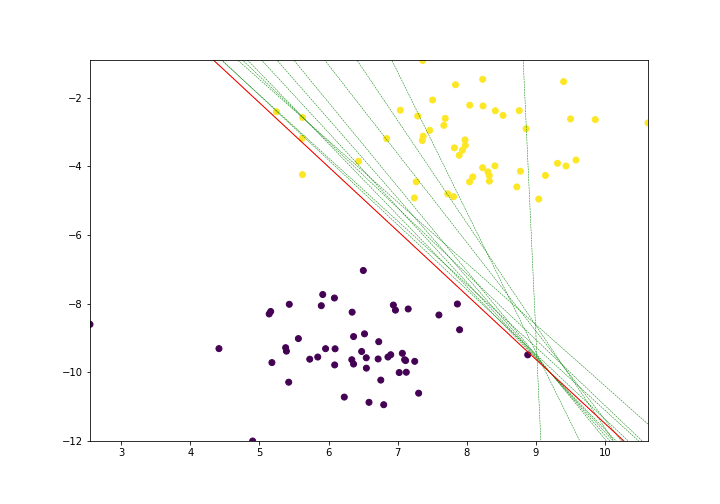

Let's run our algorithm for 35 epochs.

lines = trainPerceptronAlgorithm(X, y, learn_rate = 0.01, num_epochs = 35)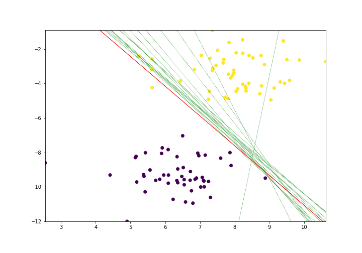

Notice the little improvement.

Let's see what happens if we increase epoch to 50

lines = trainPerceptronAlgorithm(X, y, learn_rate = 0.01, num_epochs = 50)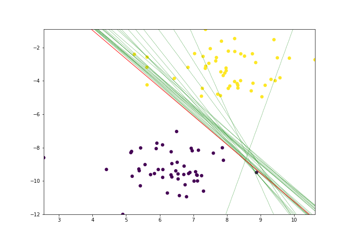

As you can see from the above "Red line" is achieving a significant accuracy as it is misclassifying only one yellow point in the dataset.

Our model is performing great on this data. Great!

Get the complete code on GitHub.